Flash floods in steep tropical basins are a result of the interplay of short-duration rainfall extremes, antecedent wetness, relief, drainage connectivity, and land-surface conditions. The present study compares the machine-learning and deep-learning techniques for flood-susceptibility mapping in the Sangu-Matamuhuri River Basin, Bandarban-Cox's Bazar, southeast Bangladesh, using a diverse geospatial and hydrometeorological benchmark. There are 250 labelled samples, 16 static GIS-like predictors, four rainfall aggregates, and a 144-step antecedent rainfall sequence. Inconsistent event timestamps, spatially incoherent validation blocks, and disagreement between the rainfall sequences and their reported cumulative totals were identified during a pre-modelling audit and were corrected prior to modelling. Five-fold spatial-block cross-validation and a completely withheld event were used to evaluate logistic regression, radial-basis SVM, random forest, XGBoost, multilayer perceptron, and a storm-conditioned deep learning neural network (SC-DLNN). The discrimination was weak to modest for spatial cross-validation (mean ROC-AUC 0.475-0.560; SC-DLNN 0.559 +/- 0.148), but was significantly higher for several conventional models on the withheld E03 event, with random forest achieving ROC-AUC 0.797. The cartographic figures show a high relief contrast from east to west, a concentration of historical flood sites along the Sangu-Matamuhuri drainage system, and an exploratory susceptibility pattern with high and very-high classes along major river corridors and parts of the dissected eastern basin. The 72-h rainfall, distance to stream, and 3 h rainfall was highlighted in XGBoost attribution, whereas SC-DLNN attention focused on the 24-72 h antecedent window. The overall results indicate that plausible spatial patterns should be considered in conjunction with data provenance, leakage-aware validation, calibration, and uncertainty, and not in terms of model complexity or a single good performance metric
Keywords - flood prediction; machine learning; deep learning; big data techniques; susceptibility mapping; spatial validation; Sangu-Matamuhuri River Basin; Bangladesh
Keywordsflood predictionmachine learningdeep learningbig data techniquessusceptibility mappingspatial validationSangu-Matamuhuri River BasinBangladesh
1. Introduction
Floods and flash floods are spatially complex natural hazards that are dependent on the interplay of meteorological forcing, antecedent moisture, terrain configuration, drainage connectivity, land cover, and local storage capacity. In steep tropical basins, the hydrological response time is short, so that high-intensity rainfall can be quickly translated into concentrated runoff, and the valley geometry and proximity of the channel determine where the runoff is conveyed, stored or accumulated. The nonlinear interactions make flood-susceptibility analysis an ideal application for machine-learning techniques that can incorporate a variety of geospatial and hydrometeorological data, such as digital elevation products, rainfall sequences, land-surface indicators, drainage metrics, and flood inventories (Bui et al., 2020; Mosavi et al., 2018)
The Sangu-Matamuhuri system in the south-eastern part of Bangladesh is a relevant context for this analysis as it is a rugged upland, heavily dissected drainage, monsoon rainfall and settlements are clustered along the major river corridors. Both rivers are considered to be important upland freshwater systems with a high seasonal discharge variability based on long-term streamflow research (Rudra & Alam, 2023) In Bangladesh, the watershed morphology, hydro-geomorphological factors, rainfall extremes, random forests, neural networks, recurrent models, and boosting algorithms are important for flood-susceptibility assessment in the region (Adnan et al., 2019; Ahmed et al., 2022; Zzaman et al., 2021). The present study builds on this literature by combining the spatial information displayed on the basin maps with leakage-aware validation and model interpretation.
Geographic generalization is not guaranteed by reported accuracy; adjacent observations may have the same drainage, terrain, and land-surface structure, and random partitions of the training set can be designed to give high scores to interpolating between the observations, but not to extrapolating to truly unsampled locations. If geographic dependence is suspected, then spatially structured cross-validation is needed (Islam & Chowdhury, 2024; Roberts et al., 2017; Valavi et al., 2019). Event dependence is a complementary problem, as a model can discriminate well for one storm, but not for others under different geographic or rainfall conditions. Geographic transfer and event transfer are thus assessed separately.
The same applies to the combination of heterogeneous predictor sets and rainfall sequences, where data integrity is also crucial. The identifiers of events should match the event catalogue, the spatial groups for validation should be geographically coherent, and the sequences of rainfall should have the same cumulative totals as reported. When these conditions are not met, artefacts from the construction of the datasets can be amplified by the model complexity, instead of hydrological information. Explainability tools like SHAP can highlight variables that affect fitted predictions (Lundberg & Lee, 2017) and Monte Carlo dropout can describe stochastic predictive variability (Gal & Ghahramani, 2016) but neither can make up for inappropriate validation or uncertain provenance.
The numerical data presented here is clearly identified as a synthetic training benchmark. Therefore, its 250 model records are not considered as observed inundation data from Sentinel-1 and the benchmark covariates are not considered as a fully verified empirical raster stack. Figures 1-4 are thus employed to convey geographic context, conditioning-factor structure, sampling geometry and exploratory spatial model output. If a figure is similar to an empirical GIS product, interpretation is limited to the spatial pattern that is observed in the figure, unless the benchmark offers a reproducible quantitative basis for a stronger claim. The study then assesses the ability of machine-learning and deep-learning methods to correctly classify flash-flood susceptibility in the presence of heterogeneous inputs, data-quality auditing, leakage-aware spatial validation, independent-event testing, and model interpretation.
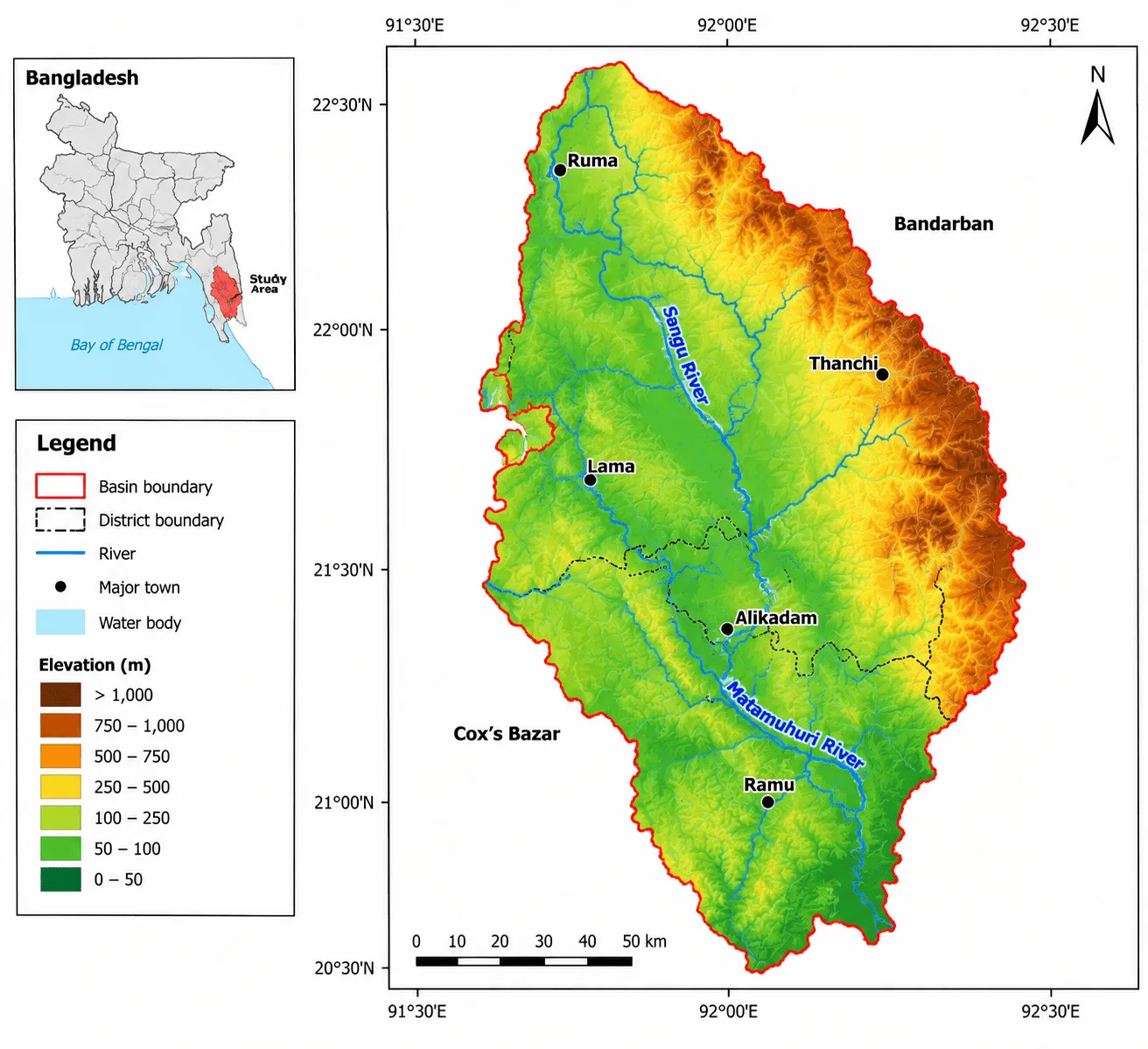
Figure 1.Study Area and Topographic Setting of the Flash Flood-Prone Basin
The three research questions that guide the analysis are: (RQ1) What spatial information is provided by the study-area, flood-inventory, conditioning-factor and susceptibility figures, and how should these patterns be interpreted in relation to the benchmark data? (RQ2) Is logistic regression, SVM, random forest, XGBoost, MLP and SC-DLNN able to consistently discriminate and classify skills in spatial-block cross-validation and completely withheld-event testing? (RQ3) What are the dominant rainfall, terrain and drainage variables for model attribution, and what is the probability stratification that can be achieved by the susceptibility classes, and how much does it overestimate the basin-wide predictive skill?
The specific objectives are: (i) to characterize the topographic and drainage setting of the Sangu-Matamuhuri basin; (ii) to examine the spatial arrangement of the historical flood inventory and analytical sample points; (iii) to relate the conditioning-factor maps to the predictor families represented in the numerical benchmark; (iv) to audit and harmonize event metadata, spatial blocks, and rainfall sequences before modelling; (v) to compare five conventional classifiers with a static-plus-BiGRU-attention SC-DLNN under common validation schemes; (vi) to quantify discrimination, class balance, probabilistic error, and uncertainty; and (vii) to interpret susceptibility zonation and feature-attribution outputs within the evidential limits of the available data..
2. Literature Review
The methods used for flood and flash-flood susceptibility modelling have gradually evolved from weighted-overlay and multi-criteria methods to machine-learning, deep-learning and explainable-AI workflows. (Zzaman et al., 2021) Validated 12 hydro-geomorphological factors in the Sangu River basin with AHP and ANP and obtained validation scores of around 0.77-0.79. That study set the stage for the regional relevance of terrain, rainfall, drainage, HAND, and land-surface controls, but did not explicitly consider spatial sample dependence or machine-learning leakage. This distinction is significant because when training and validation samples have similar geographic structure, susceptibility models can seem very accurate. Later, nonlinear learning algorithms were used more and more in Bangladesh. (Ahmed et al., 2022) validated the Deep Boost, a deep-learning neural network, and an artificial neural network on the Brahmaputra floodplain, and obtained validation AUC values of 0.917, 0.901, and 0.895, respectively, with a randomly partitioned flood inventory.
(Islam & Chowdhury, 2024) Evaluated the performance of random forest and SVM for the local-scale flash-flood susceptibility in the northeastern part of Bangladesh, and found that random forest performed well (AUC 0.964, accuracy 92.1%, kappa 0.894), along with spatial agreement analysis. (Rifath et al., 2024) expanded the problem to the hilly south-eastern region with multiple machine-learning models, 12 flood-conditioning variables and climate scenarios, and (Chowdhury et al., 2025) added rainfall extremes and compared the performance of ANN, RNN, RFGB, and CatBoost in eight districts of the north-eastern region. These studies highlight the predictive ability of nonlinear models, but also illustrate that reported performance is dependent on the flood inventory, the set of predictors, spatial support, and the validation design.
Uncertainty and interpretability have also been emphasized in a parallel literature, such as the work by (Adnan et al., 2023) on the significant differences between geospatial flood-susceptibility models, and by (Pradhan et al., 2023) on model attribution using SHAP. These developments complement frameworks for evaluation that take into account discrimination, spatial transfer, uncertainty, and interpretability, in addition to accuracy.
The other methodological shortcoming is not just that a more complex architecture can get a higher AUC. Optimistic estimates of model generalization can be obtained due to spatial autocorrelation, event dependence, internally inconsistent rainfall sequences, and non-independent train-test partitions. The present study aims to fill this gap by introducing data-integrity auditing before model fitting, by decoupling the spatial-block validation from the independent-event transfer, and by viewing SHAP, permutation importance, temporal attention, and Monte Carlo dropout as diagnostics of the fitted-model behaviour, rather than as causal hydrological evidence. This design explicitly represents the structure of the validation and the provenance of the data in the scientific inference.
Table 1. Summary of Representative Studies on Flood and Flash-Flood Susceptibility Modelling Using Machine Learning, Deep Learning, and Related Spatial Approaches
Study
Study area/data context
Methods
Reported result
Relevance to present study
(Zzaman et al., 2021)
Sangu River basin, Bangladesh
AHP; ANP; 12 hydro-geomorphological factors
Validation approximately 0.77-0.79
Strong regional hydro-geomorphic basis; no ML leakage analysis
(Ahmed et al., 2022)
Brahmaputra floodplain, Bangladesh
Deep Boost; DLNN; ANN
AUC 0.917, 0.901, 0.895
High predictive performance under random 70/30 partition; spatial transfer not separately tested
(Adnan et al., 2019)
Bangladesh geospatial flood modelling
Four standalone/hybrid ML models; uncertainty framework
Cross-model spatial association reported as 0.62-0.91
Shows model-choice uncertainty and the need for uncertainty-aware interpretation
(Islam & Chowdhury, 2024)
Northeastern Bangladesh
RF; SVM
RF AUC 0.964; accuracy 92.1%; kappa 0.894
Adds spatial agreement assessment at local scale
(Rifath et al., 2024)
Hilly southeastern Bangladesh
Multiple ML models + climate scenarios; 12 factors
Random forest reported as most accurate; future high-risk area increases
Direct regional relevance and climate-sensitivity perspective
(Chowdhury et al., 2025)
Eight districts, northeast Bangladesh
ANN; RNN; RFGB; CatBoost; rainfall extremes
400 flood/non-flood points; five susceptibility classes
Integrates rainfall extremes with nonlinear susceptibility modelling
(Pradhan et al., 2023)
Jinju, South Korea
Explainable AI / SHAP
Reported accuracy 88.4%
Demonstrates the value of attribution but not causal inference
3. Study Area
The study area is the Sangu-Matamuhuri River Basin in the Bandarban-Cox's Bazar region of the southeast of Bangladesh. The topographic gradient of the analytical domain represented in the benchmark is quite pronounced, with lower elevation terrain mainly along the central, western and southern valley systems, and higher, more dissected uplands along the eastern and northeastern margins (Figure 1). The Sangu River is the main north-central drainage and the Matamuhuri River drains the central and southern parts of the basin. These valley and river systems are located near major settlements, such as Ruma, Thanchi, Lama, Alikadam and Ramu, highlighting the relevance of flood exposure along channels. The topographic structure illustrated in Figure 1 is hydrologically significant because the steep relief around confined valleys can reduce the runoff concentration time and enhance the difference between the hillslope source areas and channel-receiving areas. The Chittagong Hill Tracts are also gradually moving towards the Cox's Bazar lowlands, further accentuating an upstream-downstream gradient in terrain and drainage organization. Figure 1 thus serves as the physical reference for the interpretation of the drainage-proximity, flow-accumulation, wetness, land-surface and rainfall variables that are used later in the modelling framework.
4. Data and Methods
4.1 Data Sources and Conditioning Factors
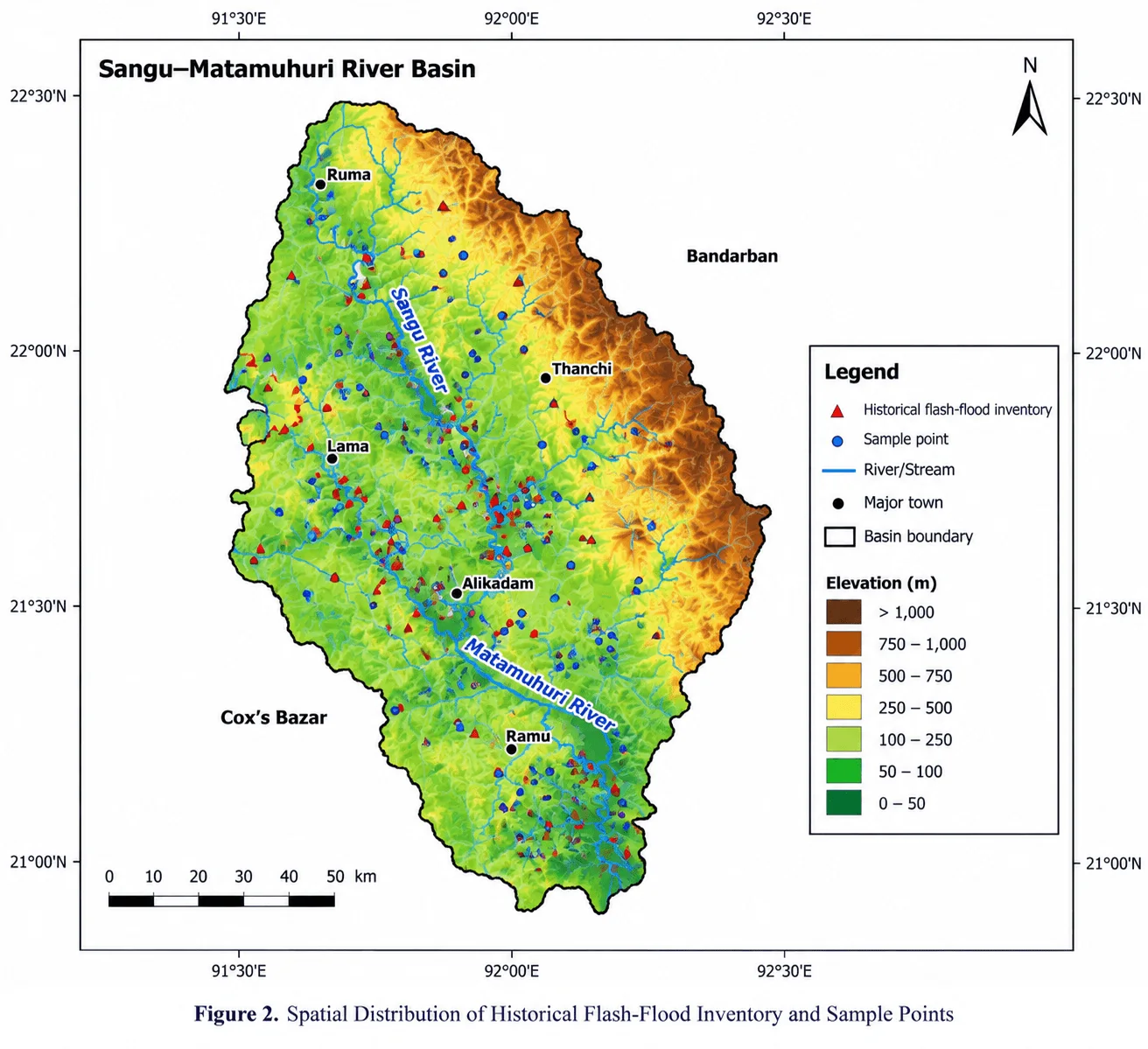
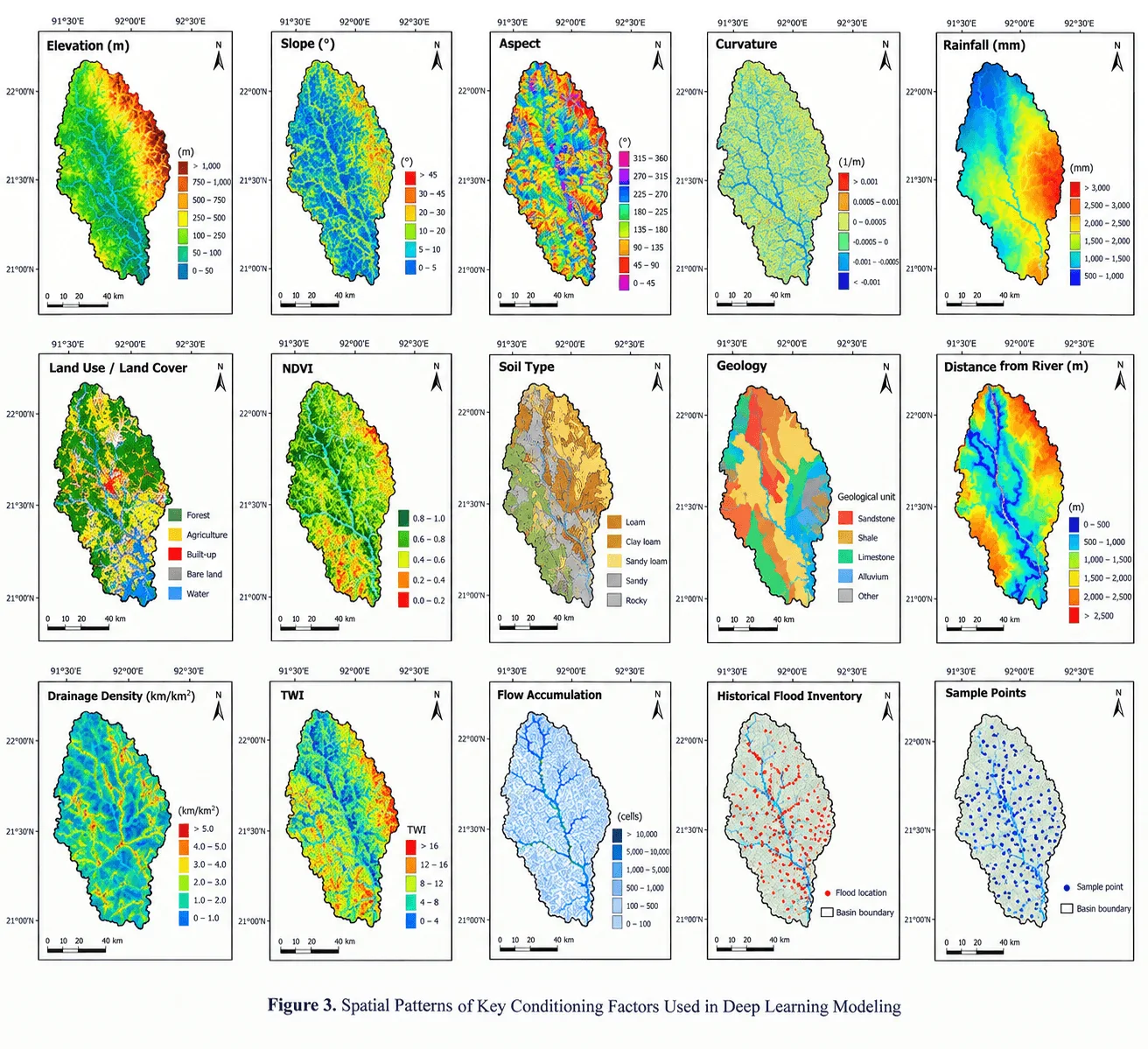
The analysis is performed on two files from the Sangu-Matamuhuri Flood Susceptibility Dataset v1.0 package: an ANN table (250 rows x 28 columns) and an SC-DLNN table (250 rows x 172 columns). The benchmark includes seven metadata fields, 16 static GIS-like predictors, four rainfall aggregates, a binary flood label, and in the sequence file, 144 rainfall values at 30-minute intervals for the previous 72 hours. There are 84 flood samples and 166 non-flood samples documented in the class distribution (33.6% and 66.4%, respectively). These sample-level records are presented in the context of the spatial distribution of the flood inventory, the analytical sample locations, and the major terrain, hydrological, land-surface, soil/geological, and rainfall factor families in the larger workflow, as shown in Figures 2 and 3.
Figure 2.Spatial Distribution of Historical Flash-Flood Inventory and Sample PointsFigure 3.Spatial Patterns of Key Conditioning Factors Used in Deep Learning Modeling
The cartographic layers and the numerical benchmark are not the same data object but they are related. Figure 3 shows the elevation, slope, aspect, curvature, rainfall, land use/land cover, NDVI, soil type, geology, distance from river, drainage density, TWI, flow accumulation, flood inventory and sample points. The model table, on the other hand, has synthetic numerical variables such as elevation, slope, TRI, plan curvature, profile curvature, TWI, SPI, HAND, flow accumulation, drainage density, distance to stream, NDVI, built fraction, forest fraction, clay percentage, and sand percentage, as well as rainfall aggregates. As a result, aspect and geology are treated as contextual cartographic layers (not separate benchmark predictors), and TRI, SPI, HAND, and neighborhood land-cover fractions are numerical benchmark variables that are not shown as individual Figure 3 panels.
This separation avoids the false one-to-one correspondence between the map panels and model columns. Elevation and slope distinguish high-relief source areas from lower valley floors; aspect and curvature describe the orientation and local convergence or divergence of terrain; distance to river, drainage density, TWI and flow accumulation describe proximity and connectivity to runoff pathways; land cover and NDVI describe surface condition and vegetation; soil and geology provide infiltration and substrate context, and rainfall provides meteorological forcing. The four rainfall aggregates and the 16 static benchmark variables were used in conventional models. The 16 static variables were placed in the SC-DLNN static branch, and the 144-step rainfall sequence was placed in the temporal branch, thus eliminating the duplication of the aggregate rainfall information across the two branches. Figure 2 also indicates that flood-inventory locations are not evenly distributed, with the red flood points focusing on the Sangu and Matamuhuri trunk channels and connected valleys, while the blue analytical sample points are more representative of the hillslopes, tributaries and interfluves. Geographically structured validation is motivated by this spatial dependence. The development data was therefore subjected to predictor screening, which resulted in a maximum VIF of 2.048 and a maximum absolute Spearman correlation of 0.590, which were not considered to be severe.
Table 2. Conditioning-Factor Families, Relationship to Figure 3, Data Provenance, Resolution, and Rationale for Inclusion
Synthetic benchmark; intended empirical source: DEM and terrain derivatives
Sample-level model values; basin-scale cartographic layers shown for context
Represents relief, steepness, roughness, terrain orientation, and local convergence/divergence. Aspect is shown in Figure 3 but is not a separate benchmark predictor.
Hydrological terrain
TWI; SPI; HAND; flow_accum_km2; Figure 3: TWI and flow accumulation
Benchmark metadata and cartographic inventory/sample layers
Point support with event identifiers
Defines the response variable, sampling geometry, and validation structure; these are not predictor variables.
4.2 Data Preprocessing and Sampling Strategy
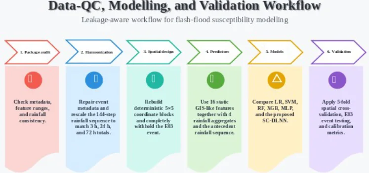
Data integrity was assessed before model fitting. The audit covered missingness, duplicate sample IDs, event-time consistency, geographic coherence of block identifiers, agreement between the 144-step rainfall sequences and their 3 h, 24 h, and 72 h cumulative variables, and multicollinearity in the development data. No missing values or duplicate IDs were detected, but three structural inconsistencies required correction. First, only 1 of 250 original timestamps fell within the event period associated with its event identifier. Because timestamps were metadata rather than predictors, the original values were retained for audit purposes, and the working metadata were aligned to catalogue peak times. Target labels and predictive covariates were unchanged. Second, the original block identifiers were not geographically compact.
Mean pairwise separation within original blocks was 0.435 degrees. The observed latitude-longitude extent was therefore divided into five equal bins in each dimension, producing 25 deterministic coordinate blocks and reducing mean within-block separation to 0.0846 degrees. These cells serve only as leakage-control groups, not hydrological sub-basins. Third, the 144-step rainfall sequences were inconsistent with the aggregate rainfall fields. Sequence-derived 3 h, 24 h, and 72 h totals correlated only 0.029, 0.018, and -0.003 with the supplied aggregates, with mean absolute discrepancies of 25.43, 124.40, and 469.23 mm. The 0-3 h, 3-24 h, and 24-72 h segments were therefore rescaled to R3, R24 - R3, and R72 - R24, respectively, while preserving within-window temporal shape.
Here, r_(i,t) is the original rainfall value for sample i at timestep t, j denotes a non-overlapping temporal window, and T_(i,j) is the aggregate rainfall assigned to that window. After rescaling, maximum reconstruction error for the 3 h, 24 h, and 72 h totals was below 5 x 10^-13 mm. The harmonized sequence and metadata were used thereafter.
E03_Regional was completely withheld from scaling, training, model selection, and threshold selection. The remaining 183 samples from E01, E02, and E04 formed the development set. Five-fold Stratified Group K Fold cross-validation used reconstructed spatial block as the grouping variable and flood status for stratification where feasible. Identical folds were used for all models. Spatial-block cross-validation therefore tests geographic transfer, while untouched E03 provides a complementary event-transfer test. Performance was evaluated using ROC-AUC and PR-AUC; balanced accuracy, precision, recall, F1-score, and MCC; and Brier score. For E03, each decision threshold was selected exclusively from development out-of-fold predictions by maximizing F1 over 0.10-0.90. Non-parametric bootstrap resampling provided 95% confidence intervals for ROC-AUC and PR-AUC.
4.3 Conceptual Framework
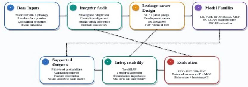
The conceptual framework treats susceptibility modelling as a sequence of inferential controls rather than an algorithm-selection exercise. Predictor provenance and consistency are checked first; leakage-aware sampling then separates geographic from event transfer. Conventional baselines and the SC-DLNN use the same spatial folds, after which discrimination, calibration, attribution, and uncertainty are interpreted within the limits of the synthetic benchmark. This ordering prevents plausible maps or favourable single-split scores from being treated as sufficient evidence of basin-wide predictive skill.
4.4 Proposed Machine Learning / Big Data Architecture
Five conventional algorithms represented complementary model families: class-weighted logistic regression, class-weighted radial-basis SVM, random forest, XGBoost, and a two-hidden-layer MLP. Hyperparameters were fixed before independent-event evaluation and kept deliberately parsimonious for the small development sample.
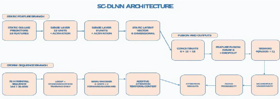
The SC-DLNN contains static and temporal branches. Sixteen standardized static predictors pass through dense layers of 12 and 6 units. The 144-step rainfall sequence is log1p-transformed, standardized using training data, and encoded by a bidirectional GRU with six hidden units per direction. Additive attention forms a 12-dimensional storm context. This is concatenated with the six-dimensional static representation, passed through an eight-unit fusion layer, and mapped to a sigmoid probability. Weighted binary cross-entropy addresses class imbalance and AdamW performs optimization.
Early stopping used the validation Brier score rather than training accuracy. The median best epoch across the five spatial folds was five; this fixed epoch count was used to fit the frozen final SC-DLNN on all development samples before E03 evaluation.
Table 3. Hyperparameters and Training Configuration of the Proposed Deep Learning Neural Network Architecture and Benchmark Models
Model
Configuration
Logistic regression
StandardScaler; C=1.0; balanced class weights; max_iter=3000
SVM (RBF)
StandardScaler; C=2.0; gamma=scale; balanced class weights; probability calibration enabled
Random forest
800 trees; max_depth=8; min_samples_leaf=3; max_features=sqrt; balanced class weights
Evaluation distinguished discrimination, classification, probabilistic error, geographic transfer, and event transfer. ROC-AUC and PR-AUC summarized threshold-independent discrimination; balanced accuracy, precision, recall, F1-score, and MCC summarized classification; and Brier score quantified probability error. E03 thresholds were selected only from development out-of-fold predictions, and bootstrap resampling generated 95% confidence intervals for ROC-AUC and PR-AUC.
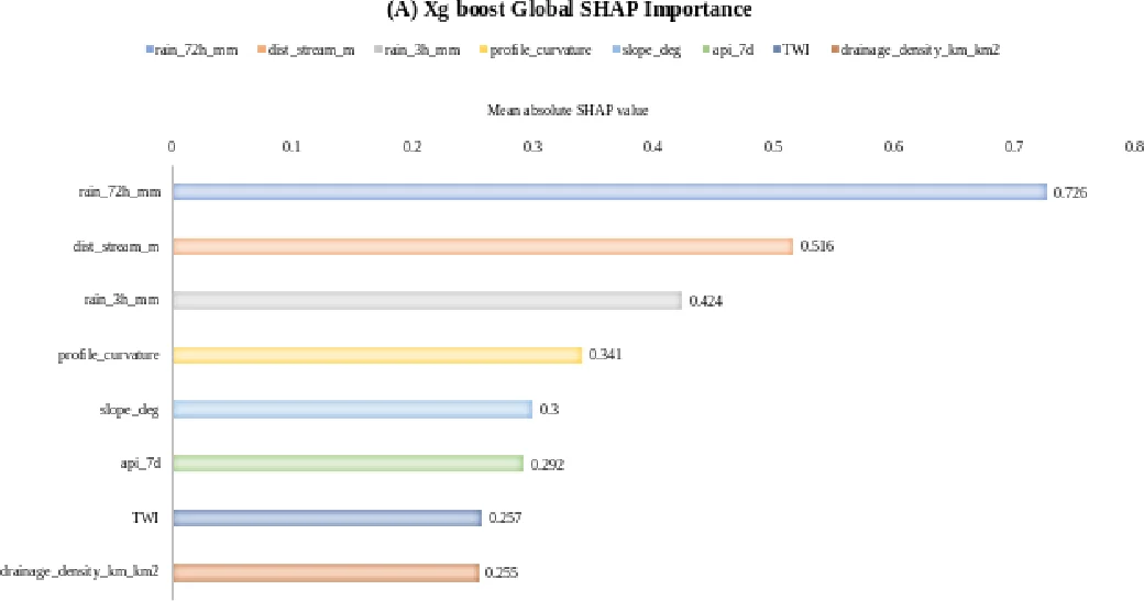
We interpreted XGBoost on E03 using TreeSHAP. Global importance was summarized by mean absolute SHAP value, and leading-predictor distributions were examined for attribution structure. SHAP values are treated as fitted-model attribution rather than causal hydrological effects.
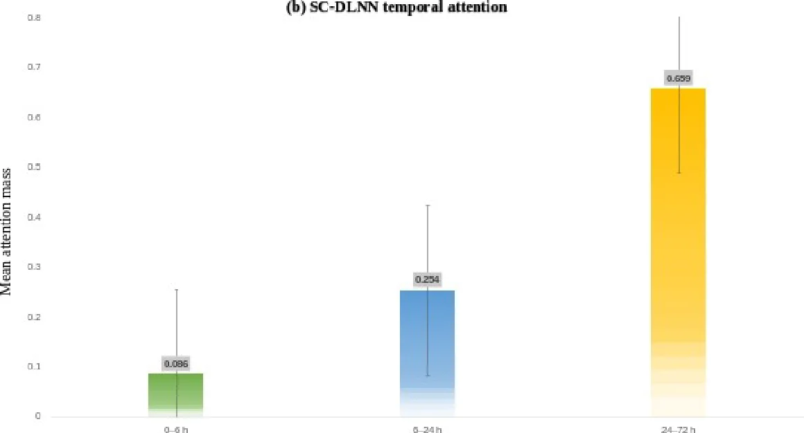
For the SC-DLNN, attention weights were aggregated into 0-6 h, 6-24 h, and 24-72 h windows. We assessed static-variable sensitivity by the decrease in E03 ROC-AUC after permuting one standardized predictor. Predictive uncertainty was approximated with 20 Monte Carlo dropout passes using the standard deviation of predicted probabilities.
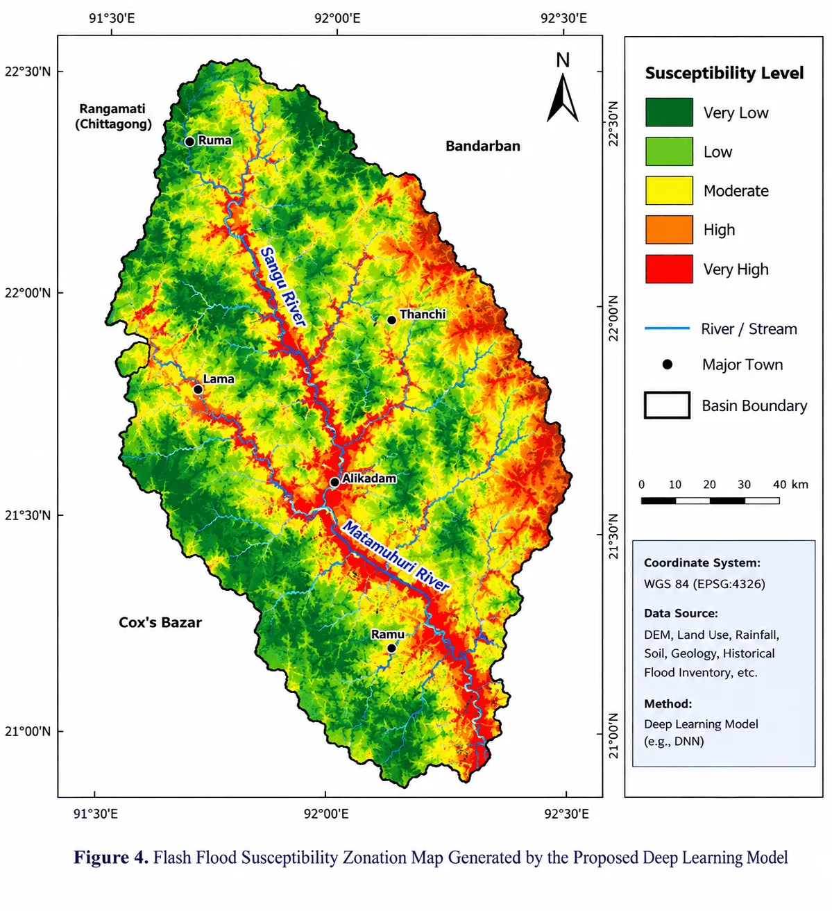
The benchmark lacks a fully documented continuous empirical predictor stack and independent pixel-level flood mask from which basin-wide accuracy, susceptible area, or flood-pixel capture rates can be reproduced. Figure 4 is therefore treated as exploratory cartographic output. Quantitative validation is restricted to the sample-level benchmark and held-out event predictions, preventing map detail from being interpreted as stronger evidence than the data support.
Figure 4.Data Preprocessing, Feature Engineering, and Sampling Workflow for Model Development
5. Results
5.1 Data Audit and Validation Context
After harmonization, all 250 samples and all 20 static/aggregate predictors were retained. The development events E01, E02, and E04 contributed 183 samples, while E03 remained completely withheld and contained 67 samples, including 24 flood and 43 non-flood observations. Flood prevalence ranged from 27.9% in E04 to 37.5% in E02. Mean 72 h rainfall was comparatively similar across event groups (184.2-192.1 mm), indicating that event identity did not simply partition the benchmark into low- and high-rainfall regimes. The spatial patterns in Figures 2 and 3 further show that flood observations and hydrological controls are geographically structured, supporting the need for spatially grouped validation. Predictor screening indicated low-to-moderate rather than severe redundancy. The largest VIF was 2.048 for 24 h rainfall, and the maximum absolute pairwise Spearman correlation was 0.590; no predictor was therefore removed on multicollinearity grounds. Consequently, the weak geographic discrimination reported below cannot be attributed simply to an unstable set of highly collinear predictors. It is more plausibly interpreted in the context of the small sample, synthetic data-generating structure, spatial and event dependence, and limited transferable signal.
5.2 Quantitative Model Performance Metrics
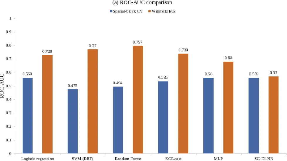
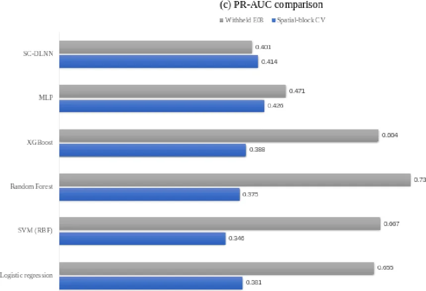
Table 4 shows that no model achieved consistently strong performance under five-fold spatial-block cross-validation. Mean ROC-AUC ranged from 0.475 for the RBF SVM to 0.560 for the MLP; logistic regression and the SC-DLNN both reached 0.559, indicating little separation among the leading models. The ranking changed across complementary metrics. The MLP produced the highest mean PR-AUC (0.426), balanced accuracy (0.521), and MCC (0.063), whereas logistic regression yielded the highest F1-score (0.381). The SVM achieved the lowest Brier score (0.222) but F1-score and MCC values of zero at the common 0.50 threshold, illustrating that comparatively low probabilistic error did not translate into useful minority-class separation. Random forest and XGBoost also produced negative MCC values (-0.108 and -0.060). Taken together, the metric profile provides no evidence of a clearly dominant model for geographic transfer.
Table 4. Quantitative Performance Metrics of All Evaluated Models for Flash Flood Susceptibility Prediction
Model
ROC-AUC
PR-AUC
Balanced acc.
F1
MCC
Brier
Logistic regression
0.559 +/- 0.051
0.381 +/- 0.089
0.501 +/- 0.031
0.381
0.003
0.275
SVM (RBF)
0.475 +/- 0.063
0.346 +/- 0.048
0.500 +/- 0.000
0.000
0.000
0.222
Random Forest
0.494 +/- 0.136
0.375 +/- 0.172
0.457 +/- 0.052
0.053
-0.108
0.234
XGBoost
0.535 +/- 0.110
0.388 +/- 0.165
0.472 +/- 0.119
0.232
-0.060
0.288
MLP
0.560 +/- 0.098
0.426 +/- 0.107
0.521 +/- 0.042
0.130
0.063
0.223
SC-DLNN
0.559 +/- 0.148
0.414 +/- 0.091
0.514 +/- 0.032
0.087
0.029
0.238
5.3 ROC Curves and AUC-Based Discrimination
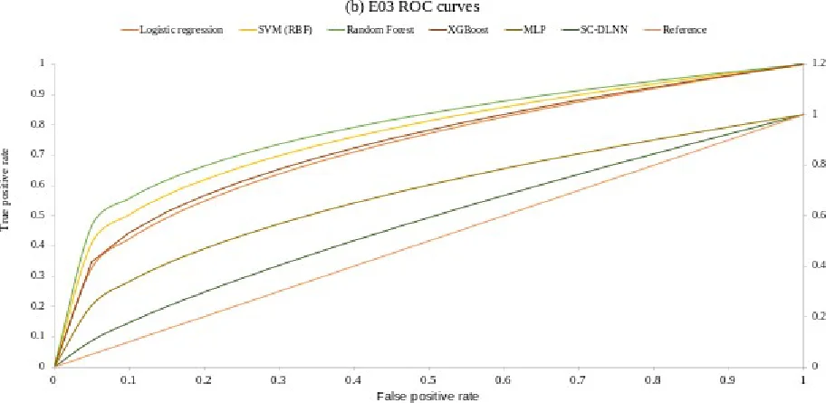
Independent-event testing produced a markedly different performance pattern. On the completely withheld E03 event, random forest achieved the highest ROC-AUC (0.797; 95% bootstrap CI 0.679-0.894) and the lowest Brier score among the conventional models (0.194). SVM followed with ROC-AUC 0.770, XGBoost with 0.739, logistic regression with 0.728, and MLP with 0.680. XGBoost nevertheless provided the strongest threshold-dependent classification on E03, with F1 = 0.618 and MCC = 0.343, despite not having the highest ROC-AUC. The SC-DLNN achieved ROC-AUC 0.570 and PR-AUC 0.401. The models were therefore ranked differently by discrimination, classification, and probabilistic metrics, demonstrating why performance should be interpreted multidimensionally rather than through a single score. Figure 8 makes the validation contrast explicit: event-holdout ROC-AUC values are substantially higher than spatial-block means for several conventional models, whereas the SC-DLNN shows little improvement. The editable ROC traces were reconstructed from the reported AUC statistics rather than from raw point-wise prediction scores, so their exact curve geometry is illustrative; the defensible quantitative evidence is the reported AUC ordering and confidence intervals. The central result is therefore the divergence between event transfer and geographic transfer: strong discrimination on one withheld event does not imply robust performance across geographically separated parts of the basin.
5.4 Model Performance Comparison
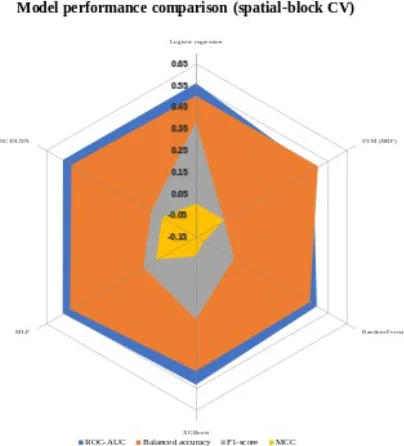
Figure 9 reinforces the cross-validation result by placing ROC-AUC, balanced accuracy, F1-score, and MCC on a common model-by-model display. ROC-AUC and balanced accuracy remain close to chance-to-modest levels across all six models, while F1-score and MCC are substantially lower and are zero or negative for several algorithms. The figure therefore shows that modest ranking ability was not accompanied by reliable threshold-based separation of flood and non-flood samples. Under this validation design, increasing algorithmic complexity from linear and tree-based models to the SC-DLNN did not yield a systematic gain in geographic transfer.
5.5 Confusion Matrix and Classification Behaviour
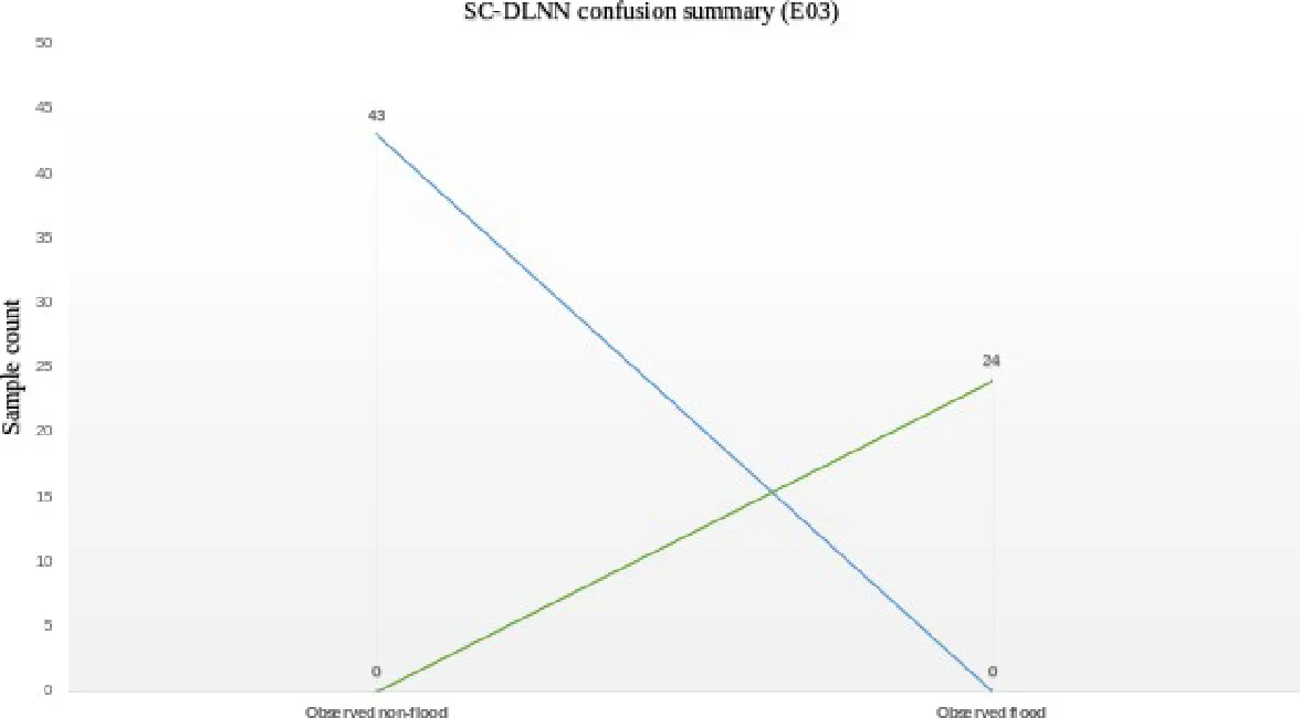
The SC-DLNN confusion pattern on E03 explains why its F1-score requires cautious interpretation. Holdout probabilities were compressed between 0.500 and 0.533 (mean 0.522, SD 0.0065), whereas the threshold selected from development out-of-fold predictions was 0.10. Consequently, all 67 E03 observations were classified as flood: all 24 observed floods were true positives, but all 43 non-flood observations were false positives. Recall was therefore 1.00, specificity was 0, balanced accuracy was 0.50, and MCC was 0.00. Figure 10 demonstrates that the apparently moderate F1-score of 0.527 reflects threshold collapse rather than useful class discrimination.
5.6 Susceptibility Zonation Map
Figure 4 presents an exploratory basin-wide susceptibility visualization with five ordinal classes. The dominant spatial pattern is the development of high and very-high susceptibility corridors along the Sangu and Matamuhuri rivers and connected tributary valleys. Additional high-susceptibility patches occur across parts of the steep, dissected eastern and central basin, whereas low and very-low classes are more extensive across western and southwestern interfluves and areas farther from the principal drainage network. Moderate susceptibility generally forms transition zones between these lower-susceptibility areas and channel- or slope-associated high-susceptibility zones. The pattern is hydrologically plausible because it corresponds qualitatively with the drainage-proximity, flow-accumulation, wetness, relief, and rainfall gradients shown in Figure 3.
The cartographic coherence of Figure 4 should not be interpreted as independent evidence of operational hazard skill. The benchmark used for model evaluation does not provide a fully documented continuous empirical predictor stack and independent pixel-level flood mask from which basin-wide accuracy, susceptibility-class area, or flood-pixel capture rates can be reproduced. In addition, the SC-DLNN showed weak spatial-block discrimination. Figure 4 is therefore used to discuss the spatial pattern assigned by the model, not to establish that the mapped classes are empirically correct across the full basin.
5.7 Susceptibility Class Distribution
Table 5 provides a separate point-level assessment of probability stratification using the 67 E03 XGBoost holdout predictions. The very-low and low classes contain 25 and 16 samples, respectively, so 41 of 67 observations (61.2%) have probabilities below 0.40. The moderate class contains 9 samples (13.4%), while the high and very-high classes together contain 17 samples (25.4%). Flood prevalence is greatest in the very-high class, where 7 of 9 samples (77.8%) are observed floods, compared with 3 of 25 (12.0%) in the very-low class. The pattern is not perfectly monotonic, however: the low and high classes each contain 50% observed floods, whereas the moderate class contains 22.2%. Thus, the class distribution shows useful separation at the probability extremes but weaker calibration and discrimination through the middle of the range.
Table 5. Sample-Level Distribution of E03 XGBoost Predictions Across Five Flash-Flood Susceptibility Classes
Class
n
Sample %
Observed flood
Predicted flood
Correct
Mean probability
Very low
25
37.3%
3
2
20
0.098
Low
16
23.9%
8
16
8
0.284
Moderate
9
13.4%
2
9
2
0.474
High
8
11.9%
4
8
4
0.703
Very high
9
13.4%
7
9
7
0.880
5.8 SHAP Feature Importance and Model Interpretability
The temporal-attention results show that the SC-DLNN assigned most of its mean attention mass to the longer antecedent period: 8.6% to 0-6 h, 25.4% to 6-24 h, and 65.9% to 24-72 h. The fitted network therefore emphasized accumulated antecedent rainfall more strongly than the immediate six-hour window. This pattern must nevertheless be interpreted cautiously because the SC-DLNN achieved weak E03 discrimination and produced nearly constant holdout probabilities. The attention distribution is consequently a description of network behaviour, not evidence of a causal rainfall-memory mechanism. Monte Carlo dropout produced a mean probability standard deviation of 0.020 (maximum 0.032), but low stochastic dispersion around nearly constant predictions does not imply high predictive information.
XGBoost attribution provides a more discriminating view of the variables used for E03 prediction. The largest mean absolute SHAP value was associated with 72 h rainfall (0.726), followed by distance to stream (0.516) and 3 h rainfall (0.424). Profile curvature (0.341), slope (0.300), 7 d antecedent precipitation index (0.292), TWI (0.257), and drainage density (0.255) formed the next tier. This ordering is hydrologically consistent with the spatial structure shown in Figures 3 and 4: rainfall provides event forcing, while stream proximity, wetness, drainage concentration, slope, and curvature influence runoff routing toward valley bottoms and channels. These SHAP values remain model-attribution statistics for the synthetic benchmark and should not be interpreted as measured causal effect sizes for the real basin.
SC-DLNN permutation analysis produced a different importance ranking. The largest decrease in E03 ROC-AUC followed permutation of HAND (0.069), followed by TRI (0.039), forest fraction (0.039), SPI (0.033), and flow accumulation (0.022). The disagreement between XGBoost SHAP attribution and SC-DLNN permutation importance is itself informative: in a weak-signal benchmark, different model classes can exploit different combinations of correlated or substitutable environmental information. Figure 11 should therefore be interpreted as evidence about fitted-model behaviour rather than as identification of a single definitive physical driver of flooding.
6. Discussion
6.1 Complexity did not overcome weak geographic signal
The principal modelling result is that additional architectural complexity did not overcome weak geographic transfer. Under spatial-block validation, all six algorithms remained within chance-to-modest discrimination, and no model simultaneously achieved strong ROC-AUC, PR-AUC, F1-score, MCC, and calibration. The SC-DLNN did not outperform the conventional models and exhibited substantial fold-to-fold variability. This result is particularly important because Figure 4 is visually coherent: high susceptibility follows major drainage corridors and parts of the dissected eastern basin, a spatial pattern that is hydrologically plausible. The contrast demonstrates that a plausible-looking susceptibility map is not equivalent to validated predictive skill; spatial inference must be supported by independent performance evidence.
This result does not imply that recurrent or attention-based architectures are intrinsically unsuitable for flash-flood prediction. Model capacity must instead match the information content and independence of the data. With 183 development samples, three development events, and synthetic predictor relationships, a two-branch neural architecture has limited opportunity to learn transferable structure. The study therefore supports a data-first interpretation: heterogeneous geospatial inputs are valuable only when their provenance, spatial support, event diversity, and validation design are adequate.
6.2 Why the validation scheme changes the scientific interpretation
The contrast between spatial-block and event-holdout performance is central to the scientific interpretation. Random forest, for example, achieved ROC-AUC 0.797 on E03 but only 0.494 under spatial cross-validation. XGBoost similarly produced the strongest E03 F1-score and MCC while remaining modest under spatial blocking. Event transfer and geographic transfer therefore answer different inferential questions. Figure 2 provides a spatial explanation for why this distinction matters: flood-inventory observations are concentrated along the main drainage network, so nearby samples can share channel position, terrain, and hydrological context. Without geographic separation, such structure can produce optimistic estimates of generalization.
This result is consistent with spatial machine-learning research showing that autocorrelated observations can yield optimistic error estimates under conventional resampling [10]. Published AUC values from Bangladesh should therefore be compared cautiously because inventories, sample sizes, predictor sets, class balance, spatial support, and validation schemes differ. Here, validation design is treated as part of the scientific result rather than as a technical detail.
6.3 Hydrological interpretation of model attribution
The spatial agreement among Figures 2-4 and the XGBoost attribution results is hydrologically interpretable. Figure 2 shows that historical flood locations are concentrated along the drainage network; Figure 3 shows connected patterns of river proximity, flow accumulation, wetness, and drainage density; and Figure 4 places many high and very-high susceptibility zones along the same river and valley corridors. XGBoost then assigns substantial attribution to 72 h rainfall, distance to stream, 3 h rainfall, slope, TWI, and drainage density. Considered together, these outputs indicate that the fitted model is using a physically plausible combination of meteorological forcing and terrain-drainage connectivity to rank susceptibility.
The strength of this interpretation is constrained by provenance and validation. The benchmark values are synthetic, and several Figure 3 panels provide contextual cartography rather than exact numerical model columns. Moreover, the SC-DLNN concentrates attention in the 24-72 h window even though its E03 probabilities are nearly constant and its ROC-AUC is only 0.570. SHAP, attention, permutation importance, and visual agreement among maps can therefore support model diagnosis but cannot independently validate watershed processes. An empirical implementation should compare these attribution patterns with observed storm hyetographs, gauge or GPM rainfall, discharge response, remotely sensed flood extent, and independent spatial flood inventories.
6.4 Data-integrity auditing as a substantive methodological result
The pre-modelling audit materially improved the internal reliability of the benchmark. Event timestamps did not align with their catalogue labels, the original spatial blocks were geographically diffuse, and the 144-step rainfall sequences failed to reproduce their own 3 h, 24 h, and 72 h cumulative totals. These are substantive methodological problems rather than cosmetic data issues: incorrect event metadata can invalidate event-based testing, incoherent blocks can fail to control spatial dependence, and inconsistent rainfall sequences can cause temporal models to learn construction artefacts instead of storm information. Correcting these inconsistencies before modelling was therefore integral to the inferential validity of the analysis.
The corrections were deliberately conservative. Event-time metadata were aligned without changing target labels, coordinate blocks were reconstructed using a deterministic spatial rule, and rainfall sequences were rescaled within non-overlapping windows while preserving their supplied within-window temporal shape. These operations improved internal consistency but did not transform synthetic records into empirical observations. The harmonized files should therefore be regarded as a reproducible methodological benchmark rather than as a substitute for observed flood inventories and independently extracted raster predictors.
6.5 Implications for an empirical Sangu-Matamuhuri study
An empirical Sangu-Matamuhuri implementation should retain the leakage-aware validation architecture while replacing the synthetic inputs with a version-controlled geospatial stack. Figure 3 provides a useful template: DEM and terrain derivatives, rainfall, land use/land cover, NDVI, soil and geological context, drainage distance, drainage density, TWI, flow accumulation, and independently mapped flood occurrences. The numerical model could additionally retain HAND, SPI, TRI, and antecedent rainfall sequences. Flood masks should be event specific, temporally matched to rainfall, and independently validated; sample design should reduce spatial clustering; and validation blocks should, where possible, be informed by observed spatial autocorrelation or hydrological structure rather than an arbitrary grid.
With such data, Figure 4 could be converted from an exploratory visualization into a reproducible empirical susceptibility product. A final frozen model could be applied cell by cell to a documented predictor raster stack, after which susceptibility-class area, flood-pixel capture rate, false-positive clustering, calibration by class, and spatial uncertainty could be quantified. These quantities are not reported in the present study because the underlying empirical raster stack and independent pixel-level flood mask are not available. Maintaining this distinction is essential to the methodological defensibility of the manuscript.
6.6 Limitations
Several limitations define the study. The numerical benchmark is synthetic and cannot establish operational skill for the real basin. Only 250 labelled samples are available, with 183 used for development, limiting stable spatial generalization for a recurrent architecture. The 5 x 5 validation blocks are coordinate based rather than derived from observed autocorrelation or hydrological sub-basins, and E03 contains only 67 observations, producing wide confidence intervals. Figures 1-4 convey meaningful spatial patterns, but the package does not provide fully documented empirical raster provenance for independent cell-level reproduction. Finally, Table 5 summarizes XGBoost point probabilities rather than basin-area proportions. These constraints limit empirical interpretation but not the methodological findings on auditing, validation sensitivity, and transparent model interpretation.
7. Conclusion
This study evaluated machine-learning and deep-learning approaches for flash-flood susceptibility analysis in the Sangu-Matamuhuri River Basin using a leakage-aware, audited benchmark together with basin-scale cartographic figures. The maps establish a physically coherent geographic setting: high relief is concentrated mainly in the eastern and northeastern basin, historical flood locations cluster along the Sangu-Matamuhuri drainage system, and the conditioning-factor panels show strong spatial heterogeneity in terrain, rainfall, land surface, wetness, drainage proximity, and flow accumulation. Before modelling, the benchmark required correction of event-time metadata, spatial grouping, and rainfall-sequence consistency, demonstrating that data integrity is a prerequisite for credible machine-learning evaluation.
Model performance depended strongly on the validation design. Spatial-block cross-validation produced only weak-to-modest discrimination for all methods (mean ROC-AUC 0.475-0.560; SC-DLNN 0.559 +/- 0.148), whereas several conventional models performed substantially better on the completely withheld E03 event. Random forest achieved the highest E03 ROC-AUC (0.797), while XGBoost produced the strongest E03 F1-score (0.618) and MCC (0.343). The SC-DLNN did not demonstrate a reproducible advantage and collapsed to an all-positive classification at its development-derived threshold. The results therefore provide no evidence that architectural complexity alone improved transferable predictive skill.
The spatial outputs are informative only when interpreted alongside these validation results. Figure 4 places high and very-high susceptibility mainly along the Sangu and Matamuhuri river corridors and parts of the dissected eastern and central basin, consistent with the drainage, terrain, wetness, and rainfall structure shown in Figure 3. XGBoost attribution similarly emphasized 72 h rainfall, distance to stream, and 3 h rainfall, while SC-DLNN attention concentrated on the 24-72 h antecedent window. Table 5 shows useful point-level probability stratification at the extremes, with 77.8% observed floods in the very-high class compared with 12.0% in the very-low class, but it is not an areal summary of Figure 4.
The principal contribution is methodological as well as spatial: credible machine-learning flood studies must align data provenance, predictor definitions, figures, validation design, uncertainty, and interpretability before drawing basin-wide conclusions. A fully empirical Sangu-Matamuhuri application should repeat the workflow with documented raster predictors, event-specific flood masks, validated rainfall sequences, and spatially independent validation before reporting operational hazard zones or basin-area statistics.
8. Declarations
Funding: Funding information was not provided in the supplied manuscript or dataset package and should be completed by the authors before submission.
Conflict of interest: The supplied manuscript states that the authors declare no competing interests.
Ethics approval: Not applicable. The analysis uses geospatial-style benchmark data and does not involve human participants or animals.
Data availability: The analyses are based on the supplied Sangu-Matamuhuri Flood Susceptibility Dataset v1.0 package. The package documentation identifies the values as synthetic. Before journal submission, the authors should archive the original package, harmonized benchmark tables, spatial folds, predictions, and figure-source workbook in a persistent repository and cite the resulting DOI or accession.
Code availability: The analysis scripts used to audit, harmonize, fit the baseline models and SC-DLNN, calculate SHAP/uncertainty diagnostics, and generate figures accompany this manuscript package. Versioned dependencies should be archived with the data at submission.
Author contributions: CRediT roles and author order must be completed by the authors; these details cannot be inferred from the supplied files.
9. Acknowledgements
Acknowledgement information was not provided in the supplied manuscript. The authors should add any institutional, technical, data-access, or individual acknowledgements required by the target journal before submission.
Figure 5.Conceptual Framework for Deep Learning-Based Flash Flood Susceptibility Assessment in a Tropical Storm RegionFigure 6.Architecture of the Proposed Deep Learning Neural Network for Flash Flood Susceptibility PredictionFigure 7.ROC-AUC Comparison under Spatial-Block Cross-Validation and Withheld E03 Event ValidationFigure 8.ROC Curves of the Evaluated Models on the Completely Withheld E03 EventFigure 9.Predictive Performance under Spatial-Block and Independent-Event ValidationFigure 10.Comparative Spatial-Block Cross-Validation Performance across ModelsFigure 11.Confusion-Matrix Summary for the Proposed SC-DLNN on the Completely Withheld E03 EventFigure 12.Flash Flood Susceptibility Zonation Map Generated by the Proposed Deep Learning ModelFigure 13.Global SHAP-Based Feature Importance for XGBoost Flash-Flood Susceptibility PredictionFigure 14.Temporal Attention Distribution of the SC-DLNN Across Antecedent Rainfall Windows
10. References
Adnan, M. S. G., Dewan, A., Zannat, K. E., & Abdullah, A. Y. M. (2019). The use of watershed geomorphic data in flash flood susceptibility zoning: A case study of the Karnaphuli and Sangu river basins of Bangladesh. Natural Hazards, 99(1), 425–448. https://doi.org/10.1007/s11069-019-03749-3
Adnan, M. S. G., Siam, Z. S., Kabir, I., Kabir, Z., Ahmed, M. R., Hassan, Q. K., Rahman, R. M., & Dewan, A. (2023). A novel framework for addressing uncertainties in machine learning-based geospatial approaches for flood prediction. Journal of Environmental Management, 326, 116813. https://doi.org/10.1016/j.jenvman.2022.116813
Ahmed, N., Hoque, M. A.-A., Arabameri, A., Pal, S. C., Chakrabortty, R., & Jui, J. (2022). Flood susceptibility mapping in Brahmaputra floodplain of Bangladesh using deep boost, deep learning neural network, and artificial neural network. Geocarto International, 37(25), 8770–8791. https://doi.org/10.1080/10106049.2021.2005698
Bui, D. T., Hoang, N.-D., Martinez-Alvarez, F., Ngo, P.-T. T., Hoa, P. V., Pham, T. D., Samui, P., & Costache, R. (2020). A novel deep learning neural network approach for predicting flash flood susceptibility: A case study at a high frequency tropical storm area. Science of the Total Environment, 701, 134413. https://doi.org/10.1016/j.scitotenv.2019.134413
Chowdhury, M. E., Islam, A. K. M. S., Zzaman, R. U., & Khadem, S. (2025). A machine learning-based approach for flash flood susceptibility mapping considering rainfall extremes in the northeast region of Bangladesh. Advances in Space Research, 75(2), 1990–2017. https://doi.org/10.1016/j.asr.2024.10.047
Gal, Y., & Ghahramani, Z. (2016). Dropout as a Bayesian approximation: Representing model uncertainty in deep learning. 48, 1050–1059.
Islam, R., & Chowdhury, P. (2024). Local-scale flash flood susceptibility assessment in northeastern Bangladesh using machine learning algorithms. Environmental Challenges, 14, 100833. https://doi.org/10.1016/j.envc.2023.100833
Lundberg, S. M., & Lee, S.-I. (2017). A unified approach to interpreting model predictions. 30, 4765–4774.
Mosavi, A., Ozturk, P., & Chau, K. (2018). Flood prediction using machine learning models: Literature review. Water, 10(11), 1536. https://doi.org/10.3390/w10111536
Pradhan, B., Lee, S., Dikshit, A., & Kim, H. (2023). Spatial flood susceptibility mapping using an explainable artificial intelligence (XAI) model. Geoscience Frontiers, 14(6), 101625. https://doi.org/10.1016/j.gsf.2023.101625
Rifath, A. R., Muktadir, M. G., Hasan, M., & Islam, M. A. (2024). Flash flood prediction modeling in the hilly regions of Southeastern Bangladesh: A machine learning attempt on present and future climate scenarios. Environmental Challenges, 17, 101029. https://doi.org/10.1016/j.envc.2024.101029
Roberts, D. R., Bahn, V., Ciuti, S., Boyce, M. S., Elith, J., Guillera-Arroita, G., Hauenstein, S., Lahoz-Monfort, J. J., Schroder, B., Thuiller, W., Warton, D. I., Wintle, B. A., Hartig, F., & Dormann, C. F. (2017). Cross-validation strategies for data with temporal, spatial, hierarchical, or phylogenetic structure. Ecography, 40(8), 913–929. https://doi.org/10.1111/ecog.02881
Rudra, A. K., & Alam, A. K. M. R. (2023). Streamflow characteristics of Sangu-Matamuhuri watershed in the southeastern part of Bangladesh. Heliyon, 9(3), e14559. https://doi.org/10.1016/j.heliyon.2023.e14559
Valavi, R., Elith, J., Lahoz‐Monfort, J. J., & Guillera‐Arroita, G. (2019). block CV: An r package for generating spatially or environmentally separated folds for k ‐fold cross‐validation of species distribution models. Methods in Ecology and Evolution, 10(2), 225–232. https://doi.org/10.1111/2041-210X.13107
Zzaman, R. U., Nowreen, S., Billah, M., & Islam, A. K. M. S. (2021). Flood hazard mapping of Sangu River basin in Bangladesh using multi-criteria analysis of hydro-geomorphological factors. Journal of Flood Risk Management, 14(3), e12715. https://doi.org/10.1111/jfr3.12715
CITE THIS ARTICLE
Islam, M. M. (2026). Analyzing the Role of Machine Learning in Predicting Natural Disasters: A Case Study on Flood Prediction Using Big Data Techniques. https://www.researchbymainul.com/article/16ca42a6-037d-4a49-8909-ebf4b3bbb227
M. M. Islam, “Analyzing the Role of Machine Learning in Predicting Natural Disasters: A Case Study on Flood Prediction Using Big Data Techniques,” 2026. [Online]. Available: https://www.researchbymainul.com/article/16ca42a6-037d-4a49-8909-ebf4b3bbb227
Islam, M. M. (2026) ‘Analyzing the Role of Machine Learning in Predicting Natural Disasters: A Case Study on Flood Prediction Using Big Data Techniques’. Available at: https://www.researchbymainul.com/article/16ca42a6-037d-4a49-8909-ebf4b3bbb227
Islam, Md Mainul. “Analyzing the Role of Machine Learning in Predicting Natural Disasters: A Case Study on Flood Prediction Using Big Data Techniques.” 2026, https://www.researchbymainul.com/article/16ca42a6-037d-4a49-8909-ebf4b3bbb227.
Md Mainul Islam. “Analyzing the Role of Machine Learning in Predicting Natural Disasters: A Case Study on Flood Prediction Using Big Data Techniques.” (2026). https://www.researchbymainul.com/article/16ca42a6-037d-4a49-8909-ebf4b3bbb227.
Islam MM. Analyzing the Role of Machine Learning in Predicting Natural Disasters: A Case Study on Flood Prediction Using Big Data Techniques. 2026. https://www.researchbymainul.com/article/16ca42a6-037d-4a49-8909-ebf4b3bbb227
@misc{article_16ca42a6037d4a498909ebf4b3bbb227,
  title = {Analyzing the Role of Machine Learning in Predicting Natural Disasters: A Case Study on Flood Prediction Using Big Data Techniques},
  author = {Md Mainul Islam},
  year = {2026},
  url = {https://www.researchbymainul.com/article/16ca42a6-037d-4a49-8909-ebf4b3bbb227},
}
TY  - GEN
AU  - Md Mainul Islam
TI  - Analyzing the Role of Machine Learning in Predicting Natural Disasters: A Case Study on Flood Prediction Using Big Data Techniques
PY  - 2026
UR  - https://www.researchbymainul.com/article/16ca42a6-037d-4a49-8909-ebf4b3bbb227
ER  -
The importance of early diagnosis of chronic diseases will help in minimizing disease burden, reduce the outcome of patients, and decrease the cost of healthcare in the long-term. New technologies in the field of Artificial Intelligence (AI) allow applying predictive analytics to diagnose disease risk at an early stage using big data on clinical analysis. In this research, the researchers examine the capability of AI-based predictive models to identify early chronic disease through anonymized el
Sentiment Analysis is important to analyze consumer feedback especially in the social media where large amounts of data are being created every day. The paper explores how BERT (Bidirectional Encoder Representations from Transformers) a state of the art deep learning model may be used to analyze the sentiment of social media posts on consumer products. We use BERT on a customer review case study on Twitter, Instagram, and Facebook of a well-known consumer product. The analysis categorizes the se
With the increasing sophistication in cyber threat, conventional security mechanisms are in most cases not enough to guard organizations against the emerging risks. Cybersecurity has also gained a lot of strength through the use of artificial intelligence (AI) to detect and respond to threats. Threat detection models based on machine learning, predictive analytics, and automated security operations are AI-driven and allow achieving more precise detection, lowering false positives, and increasing